Using a shapefile to select a region and calculate statistics#
Shapefile is a geospatial format used by geographic information system (GIS) software to display vector data. Shapefiles can be used to define complex polygons and shapes like states, regions, ocean basins.
In this notebook we show how you can use a shapefile to select a specific region from a gridded dataset.
We will be showing two different methods using the following modules:
geopandas to read the polygons defined in the shapefile
rasterio and odc to create a gridded mask for each polygon
xarray to read the gridded model data and apply the mask
rasterstats to calculate zonal statistics on the region
from rasterstats import zonal_stats
import rasterio
import pandas as pd
import xarray as xr
import geopandas as gpd
import odc.geo.xr
import os
Here we are using the AGCD precipitation data and a shapefile of the Eastern Seaboard region.
# Filepaths
shapefile = '/g/data/hh5/tmp/blog/FebMar_ESB_MaryRiver_to_NSW_Vic_border_clip.shx'
ncfile = '/g/data/zv2/agcd/v1/precip/total/r005/01day/agcd_v1_precip_total_r005_daily_1999.nc'
ncfiles = '/g/data/zv2/agcd/v1/precip/total/r005/01day/agcd_v1_precip_total_r005_daily_*.nc'
We are using the AGCD data to calculate the mean precipitation in a region defined by the shapefile, but any other dataset covering the same region will do.
ds = xr.open_dataset(ncfile, chunks={'time': '200MB'}, decode_coords='all')
precip = ds.precip
precip
<xarray.DataArray 'precip' (time: 365, lat: 691, lon: 886)>
dask.array<open_dataset-151f7e306d0cdfd24c3c90d220556f3aprecip, shape=(365, 691, 886), dtype=float32, chunksize=(81, 691, 886), chunktype=numpy.ndarray>
Coordinates:
  * time     (time) datetime64[ns] 1999-01-01T09:00:00 ... 1999-12-31T09:00:00
  * lat      (lat) float32 -44.5 -44.45 -44.4 -44.35 ... -10.1 -10.05 -10.0
  * lon      (lon) float32 112.0 112.1 112.1 112.2 ... 156.1 156.1 156.2 156.2
    crs      int32 ...
Attributes:
    cell_methods:                  time: sum
    units:                         mm
    analysis_version_number:       3.01
    long_name:                     Daily precipitation
    number_of_stations_reporting:  6276
    standard_name:                 lwe_thickness_of_precipitation_amount
    frequency:                     daily
    length_scale_for_analysis:     80.0
    coverage_content_type:         physicalMeasurement
valid_range: [ 0. 100000.]NB I used decode_coords=’all’ so it will load the variables referred to in ‘grid_mapping’, ‘bounds’ and other attributes as coordinate variables.
Using zonal_stats#
The rasterstats package has a zonal_stats method which calculate statistics on regions defined by shapefiles.
To use zonal_stats we open the netcdf file as a raster, using rasterio, and we generate a mapping of the array dimensions to a coordinate reference system (affine). See:
https://pythonhosted.org/rasterstats/manual.html#raster-data-sources.
rasterio can read and write data in raster formats, including reading gridded datasets as raster.
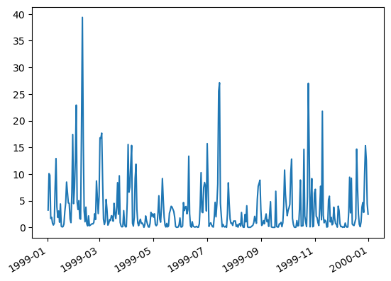
Then we loop over each timestep calling zonal_stats() and converting the resulting dictionary to a pandas dataframe.
Each dataframe is appended to a list so it can be easily concatenated later on.
zonal_stats takes as input the shapefile, the numpy array with the data from each timesteps and affine.
# added a loop to read all the arrays for each timesteps
stats_list = []
steps = len(precip.time)
with rasterio.open(f'netcdf:{ncfile}:precip') as src:
    affine = src.transform
    for i in range(1,steps+1):
        array = src.read(i)
        stats_list.append(pd.DataFrame(zonal_stats(
        shapefile, array, stats='mean', affine=affine)))
/g/data/hh5/public/apps/miniconda3/envs/analysis3-23.01/lib/python3.9/site-packages/rasterstats/io.py:335: NodataWarning: Setting nodata to -999; specify nodata explicitly
  warnings.warn(
NB by default zonal_stats returns four statistics: mean, min, max and count. Here we selected only mean.
Now we can concatenate the list of dataframe into one pandas dataframe and add the original time axis as index.
df = pd.concat(stats_list)
df.index = precip.time
df['mean']
1999-01-01 09:00:00     3.245694
1999-01-02 09:00:00    10.091568
1999-01-03 09:00:00     9.770410
1999-01-04 09:00:00     1.670065
1999-01-05 09:00:00     1.902504
                         ...
1999-12-27 09:00:00     9.743956
1999-12-28 09:00:00    15.312821
1999-12-29 09:00:00    12.549480
1999-12-30 09:00:00     4.409073
1999-12-31 09:00:00     2.465699
Name: mean, Length: 365, dtype: float64
df['mean'].plot()
<AxesSubplot:>

Creating a mask with rasterio#
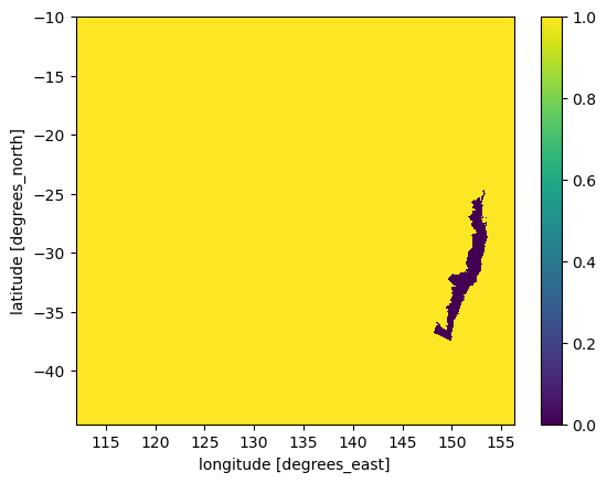
An alternative way is to create a mask for the region as a xarray DataArray with the same shape as the data. We can then use to this to select the region.
We start by opening the shapefile with GeoPandas. GeoPandas combines the capabilities of pandas and shapely, providing geospatial operations in pandas.
gdf = gpd.read_file(shapefile)
gdf.geometry
0    MULTIPOLYGON (((149.97620 -37.50516, 149.97620...
Name: geometry, dtype: geometry
There is no crs (Coordinate reference System) defined for this shapefile so I’m using the array crs which is a standard one. If the crs for the shapefile and the data array are different then you have to adapt the projection of the shapefile.
# define crs, it is not set for this shapefile
gdf.crs = "EPSG:4326"
# if this is different from the xarray data project then you need to reproject it after defining it
#gdf = gdf.to_crs(epgs='EPGS:...')
WE are using rasterio and odc-geo to create the mask. odc-geo combines geometry features from shapely with CRS from pyproj to provide projection aware Geometry. Here we use odc.geobox to provide the mapping between pixels and the geopgraphic projection.
# use rasterio and odc to create a mask
mask = rasterio.features.geometry_mask(
            gdf.geometry,
            out_shape=precip.odc.geobox.shape,
            transform=precip.odc.geobox.affine,
            all_touched=False,
            invert=False)
mask.shape
(691, 886)
We now have a mask for the selected polygon as a grid with same shape as the precipiation data. However, this is still a numpy array, so we build a xarray DataArray using precip latitude and longitude.
mask = xr.DataArray(mask, dims=('lat', 'lon'),coords=dict(
        lon=precip.lon,
        lat=precip.lat))
mask.plot()
<matplotlib.collections.QuadMesh at 0x1545b79cd7c0>

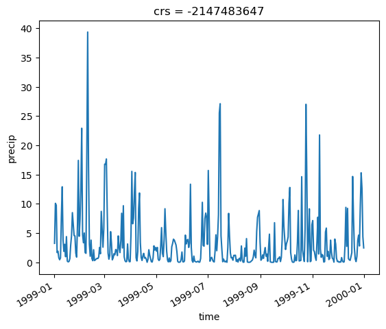
Finally we use the mask to select the data in the region of interest and calculate the mean.
pr_region = precip.where(~mask, drop=True)
meanpr = pr_region.mean(dim=['lat', 'lon'])
meanpr.plot()
[<matplotlib.lines.Line2D at 0x1545aef900d0>]

This example shows we get the same results with both methods. The first one is quite straightforward, zonal_stats does most of the work for us. It is also possible to add your own defined statistic using the add_stats argument.
Here we define a function returning the sum of the min and max.
# first define a new statistic as a function
def new_stat(array):
    """This is meaningless just to prove you can add your own calculation"""
    out = array.min() + array.max()
    return out
# then we test it on 1 timestep
with rasterio.open(f'netcdf:{ncfile}:precip') as src:
    affine = src.transform
    array = src.read(1)
    newstats = pd.DataFrame(zonal_stats(shapefile, array,
        affine=affine, stats='mean', add_stats={'mysum': new_stat}))
newstats
| mean | mysum | |
|---|---|---|
| 0 | 3.245694 | 57.436523 |
However, if we want to do a series of calculations on the region, or applying the same process to several variables, or to a multidimensional array, then creating the mask for the region once and then using it to mask the data is easier.
Another case where the mask approach is better is when we want to use the entire timeseries.
Working with multiple files#
So far we only apply this to 365 timesteps and on a relatively small region. If we want to calculate the same on the entire timeseries which consist of 121 files, it is more efficient to parallelise the computation using a dask Client.
from dask.distributed import Client
ncpus = os.environ.get('PBS_NCPUS')
c = Client(n_workers=int(ncpus))
c
/g/data/hh5/public/apps/miniconda3/envs/analysis3-23.01/lib/python3.9/site-packages/distributed/node.py:182: UserWarning: Port 8787 is already in use.
Perhaps you already have a cluster running?
Hosting the HTTP server on port 37471 instead
  warnings.warn(
Client
Client-f8f38b62-1abd-11ee-b691-00000769fe80
| Connection method: Cluster object | Cluster type: distributed.LocalCluster |
| Dashboard: /proxy/37471/status |
Cluster Info
LocalCluster
0fe5f5c4
| Dashboard: /proxy/37471/status | Workers: 2 |
| Total threads: 2 | Total memory: 9.00 GiB |
| Status: running | Using processes: True |
Scheduler Info
Scheduler
Scheduler-d51b07df-dc10-4a59-8df2-2bbfe53d46fd
| Comm: tcp://127.0.0.1:40625 | Workers: 2 |
| Dashboard: /proxy/37471/status | Total threads: 2 |
| Started: Just now | Total memory: 9.00 GiB |
Workers
Worker: 0
| Comm: tcp://127.0.0.1:44937 | Total threads: 1 |
| Dashboard: /proxy/32923/status | Memory: 4.50 GiB |
| Nanny: tcp://127.0.0.1:44193 | |
| Local directory: /jobfs/89697255.gadi-pbs/dask-worker-space/worker-jbn4l364 | |
Worker: 1
| Comm: tcp://127.0.0.1:37153 | Total threads: 1 |
| Dashboard: /proxy/32983/status | Memory: 4.50 GiB |
| Nanny: tcp://127.0.0.1:35003 | |
| Local directory: /jobfs/89697255.gadi-pbs/dask-worker-space/worker-3j9qgt2i | |
ds = xr.open_mfdataset(ncfiles, parallel=True, chunks={'time': '200MB'})
precip = ds.precip
precip
<xarray.DataArray 'precip' (time: 43981, lat: 691, lon: 886)>
dask.array<concatenate, shape=(43981, 691, 886), dtype=float32, chunksize=(81, 691, 886), chunktype=numpy.ndarray>
Coordinates:
  * time     (time) datetime64[ns] 1900-01-01T09:00:00 ... 2020-05-31T09:00:00
  * lat      (lat) float32 -44.5 -44.45 -44.4 -44.35 ... -10.1 -10.05 -10.0
  * lon      (lon) float32 112.0 112.1 112.1 112.2 ... 156.1 156.1 156.2 156.2
Attributes:
    cell_methods:                  time: sum
    units:                         mm
    analysis_version_number:       3.01
    long_name:                     Daily precipitation
    number_of_stations_reporting:  2757
    standard_name:                 lwe_thickness_of_precipitation_amount
    frequency:                     daily
    length_scale_for_analysis:     80.0
    grid_mapping:                  crs
    coverage_content_type:         physicalMeasurement
valid_range: [ 0. 100000.]The precipitation data array is ~100GB. We only use a small subset to calculate the mean, however, the data has to be first read and concatenated across the 121 files. Even using the Client, sensible chunks and parallel=True reading the data and calculating the mean took several minutes when I first run this on 2 CPUs.
As we are effectively using only a small part of the original grid, it helps pre-selecting a smaller area including the region before even concatenating the files.
First we get the region boundaries from the shapefile.
lon_min, lat_min, lon_max, lat_max = gdf.total_bounds
gdf.total_bounds
array([148.20067758, -37.50527776, 153.63833159, -24.69699057])
Then we define a function to select a region based on the boundaries.
def select_region(ds):
    ds = ds.sel(lat=slice(-38, -24), lon=slice(148, 154))
    return ds
We open the files using preprocess argument to select our region of interest from each file before concatenating them. See this blog for more information on preprocess.
%%time
ds = xr.open_mfdataset(ncfiles, parallel=True, preprocess=select_region)
precip = ds.precip.chunk({'time': '200MB'})
precip
CPU times: user 1.62 s, sys: 136 ms, total: 1.76 s
Wall time: 4.18 s
<xarray.DataArray 'precip' (time: 43981, lat: 281, lon: 121)>
dask.array<rechunk-merge, shape=(43981, 281, 121), dtype=float32, chunksize=(1460, 281, 121), chunktype=numpy.ndarray>
Coordinates:
  * time     (time) datetime64[ns] 1900-01-01T09:00:00 ... 2020-05-31T09:00:00
  * lat      (lat) float32 -38.0 -37.95 -37.9 -37.85 ... -24.1 -24.05 -24.0
  * lon      (lon) float32 148.0 148.1 148.1 148.1 ... 153.9 153.9 153.9 154.0
Attributes:
    cell_methods:                  time: sum
    units:                         mm
    analysis_version_number:       3.01
    long_name:                     Daily precipitation
    number_of_stations_reporting:  2757
    standard_name:                 lwe_thickness_of_precipitation_amount
    frequency:                     daily
    length_scale_for_analysis:     80.0
    grid_mapping:                  crs
    coverage_content_type:         physicalMeasurement
valid_range: [ 0. 100000.]NB this time we are rechunking after we concatenated the files otherwise our chunk size would be limited to the size of the selected array in each file (~10MB).
mask = mask.sel(lat=slice(-38, -24), lon=slice(148, 154))
After applying the same selection to the mask we can calculate the mean as we’ve done before.
%%time
pr_region = precip.where(~mask)
meanpr = pr_region.mean(dim=['lat', 'lon'])
meanpr = meanpr.compute()
CPU times: user 7.78 s, sys: 1.57 s, total: 9.35 s
Wall time: 4min 26s
We can see now that while it took 4 minutes of walltime, the actual execution was quite fast less than 10 seconds, just by using 2 CPUs.
Acknowledgements#
Thanks to Kim Reid for providing the use case, shapefile was created by Danielle Udy.
